Data Acquisition and Analysis System
 |
User Guide
Nuclear Science Centre,
|
|
Data Acquisition and Analysis System
|
User Guide
Nuclear Science Centre,
|
|
Table of Contents
IntroductionEvent Mode Data
The Trigger Generator
The List Processor
ADC Interfacing
Singles Data
ScalarsThe Server
The ClientChapter 5 The User InterfaceChapter 6File Menu
Online Menu
Configure Menu
Compute Menu
Project Menu
Gates Menu
Linearize Menu
Display Menu
Scales Menu
Help MenuFreedom Internals
Raw Data File format
CHAPTER 1Welcome to FREEDOM, the new Data Acquisition and Analysis System designed to support the Accelerator based experiments at Nuclear Science Centre. Some of the salient features of this system are
*Processing power that was available only on expensive workstations is achieved by combining the inexpensive IBM-PC hardware with a powerful multi-user operating system like LINUX. This enables the users from different Universities to do the off-line analysis at home with an affordable requirement of an 80486 or a Pentium having 16 MB RAM and a CDROM drive.
*This project is implemented without using any commercial software tools. The operating system used is LINUX, a unix clone developed by Linus Torvalds and a group of programmers, which is freely available on Internet. Linux runs on many hardware platforms and supports features like TCP/IP networking and X-Window Graphics.
*Handling of high data collection rates, about 400 Kbytes/sec, made possible by specially designed hardware which does part of the processing. It also helps the software to be driven by Interrupts and DMAs so that the load on CPU is minimal.
*Extensive online analysis possible without affecting the data collection speed. This is achieved by the networked design which allows two computers to share the jobs.
*Fully menu driven Graphics User Interface which is very similar to the standard window based application programmes.
The developer's policy is to encourage the users to learn the package so that any special analysis functions required can be added. Data Storage Format is explained in this documentation and to start with a small piece of code for loading it to memory is also given. The entire source code is available to the user. Designers of this package hope it will be a usefull tool for the users of NSC Accelerator and will grow further with their contributions.
System Developement
Ajith Kumar B.P. System design, Hardware modules, CAMAC driver and the Server. E.T.Subrahmaniam X-based GUI, Online Data Processing and the Offline Program. R.K.Bhowmik Guidance in System Requirements for experiments, Selection of hardware interface standards and general guidance. Jayan K.M.(A.Punithan) Assistance in fabrication of hardware modules. Acknowledgements
Documentation: Ajith Kumar B.P.
E.T.Subrahmaniam
P. V. Madhusudhana Rao.We, the development team, express our thanks to Prof. G.K.Mehta, Director, NSC, for his keen interest and support for this work. We also thank D.O.Kataria, S.K.Dutta, S.Muralithar, Pankaj Joshi, A.M.Vinod Kumar and many other research scholars and NSC staff members who tested the system and gave valuable feedback. We are indebted to Linus Torvalds and all those who contributed to the free software tools available on Internet.
Freedom is a Data Acquisition and Analysis System designed to support various experimental facilities associated with the Tandem Accelerator at Nuclear Science Centre. Before going into the details of the system let us consider the kind of data to be handled. In any accelerator based experiment the objective will be to record the signals coming from charged particle or gamma ray detectors. Each high energy particle hitting some target may cause some reaction that results in firing some of the detectors but all of these reactions or events may not be of experimental interest.
The analog signals generated by the detectors are usually processed by some logic, based on the reaction one is looking for, which selects the events of interest. For the selected events all of the detector signals are digitized and stored as a data packet. This is usually referred as the event mode data collection. An event mode data packet will have recorded data from a group of detectors generated by a particular event or reaction. The signal generated by the logic selecting the events of interest is called the event trigger.
In addition to event mode or co-related data we
need to collect data from individual detectors whenever they generate a
signal. This is the Singles Data which comes from independant detectors.
Most of the time the processing done for these signals are to generate
a histogram and record the total count received during an experimental
RUN. The system also has options to read and record scalars etc., which
collects information about the number of particles recorded by certain
detectors. The following chapters explain how Freedom collects,stores and
analyses these different types of data. First we discuss the Hardware required
to interface the data sources to the computer and then the Software which
does the job.
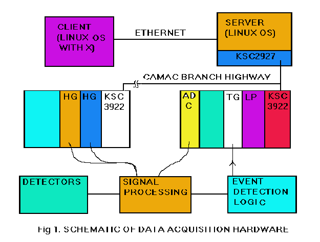
A schematic of the hardware is given in figure 1. The objective is to enable a computer to read the digitized data from the detectors. The signals from the detectors are normally analog processed using pre-amplifiers and amplifiers and then digitized by ADCs or TDCs. In our system all these data digitizers like ADCs, TDCs etc. are either CAMAC modules or NIM modules interfaced to CAMAC, in both cases they can be read by the computer by issuing a CAMAC Read Command. A Branch Highway is used for interfacing the CAMAC Crates to the computer.
CAMAC, Computer Automated Measurement And Control, is an internationally accepted modular standard for interfacing devices to a computer. Once we have all the data readable by the computer the next question is when to read them. For event mode data this has to be done according to the Event Trigger signal generated by the user defined logic. This means we need a system which digitizes and stores all the detector signals in response to an event trigger. It could be by asking the computer to read all the ADCs,TDCs etc. after digitizing each event but that method is not practical for high event rates. We need to store the data from individual events locally and transfer them to the computer in larger chunks. This has been implemented by a CAMAC List Processor module, Hytec LP1340, and a home made Trigger Generator module. These two modules and all the event mode data sources are plugged into one CAMAC Crate and work in the following manner.
When the Trigger Generator receives an Event Trigger it signals the ADCs,TDCs etc. to digitize the incoming analog signals, if the system is not busy with the previous event, and triggers the List Processor after a delay to read all the digitized data into LP's local buffer. LP has 128 Kbytes of local memory which is configured by the software into two 64Kbytes buffers. TG also keeps track of the number of events collected and interrupts the computer when it reaches the user defined limit. In response to the interrupt the computer configures LP to collect data into the alternate buffer and starts a DMA transfer from the filled buffer to the computer memory. This method allows the collection and transfer of data to go in parallel. It also frees the computer CPU for most of the time. The only job left to the CPU is to schedule a DMA transfer in response to the interrupt signal from TG. CPU time saved can be utilized in future for more elaborate event filtering and reduction of stored data.
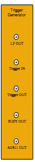
This section explains the working of the Trigger Generator module and the input and output signals associated with it.
1. Trigger Input
The Event Trigger generated by the experimentalist is given to this input. This requests the system to digitize and store that event if possible. This is a Fast NIM signal (0 to -0.8 V) and the modules senses the falling edge of the signal to take any action.
2. Trigger Output
If the system is ready to collect the event the Trigger Input is given out through the Trigger Out point. Some experiments use this signal to generate individual gate signals to trigger the ADCs etc. There is a time delay of few nanoseconds between Trigger In and Trigger Out which is caused by the ECL decision making logic.
3. AD811 Strobe Output
Since many experiments use AD811 ADCs the strobe signal required for it to start a conversion is also generated by TG module. In response to every accepted trigger input a 0 to -2 V signal of adjustable width upto 10 uS is given out.
4. LP output
The LP output from TG is connected to the List Processor Trigger Input. This is generated after a delay of about 80 uS which is the conversion time of the ADCs used. In response to this signal LP executes a list of CAMAC commands stored in it to read the event data and to re-enable the TG module for the next event.
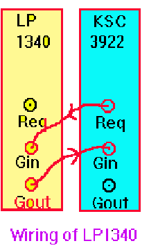
The Hytec LP1340 List Processor is an Auxiliary Crate Controller capable of executing a list of CAMAC commands stored in it, in response to an external trigger signal. The data collected during the read commands are stored into it's local memory. Since it is an ACC the Request, Grant In and Grant Out signals have to be wired properly with the main Crate Controller KSC3922. The Request signal, from the front panel LEMO of KSC3922 or LP1340, is wired to the Grant In of LP1340. The Grant Out from LP1340 is wired to the Grant In of KSC3922. This scheme gives priority to the LP module since it gets the Grant In first.
LP Trigger Input receives a low true TTL signal which is provided by the LP. Output of the TG module. Whenever LP receives a Trigger input it executes the list of stored NAF commands once and wait for the trigger again. There are many other modes in which LP can be configured but this is the way in which Freedom uses it.
The CAMAC ADCs like AD811 can be plugged into the Crate where LP & TG modules are located. The Canberra 8075 NIM ADCs can be interfaced by using the home-made CAN4 modules. This CAMAC module has four FRC connectors on the front panel which are connected to the ADCs. The data can be read by issuing F0.Ai (i= 0 to 3) commands and data accepted signal is given to all ADCs by an F10.A0 command. It also supports an F1.A0 command to provide a bit pattern indicating the availability of converted data in each ADCs.
In addition to the event mode data there are certain signals to be digitized and stored whenever they are available. Freedom handles them using the home-made Histogram Generator modules. This module along with Canberra 8075 ADC module digitizes and creates a histogram of it in the module itself. The computer reads the histogram whenever it is required for storing or displaying. The histogram generators can be located in any Crate on the Branch Highway. A 26 pin FRC connector from the rear side of HG is connected to the Data Out connector of Canberra 8075.
Freedom also supports reading and displaying of values from scalar modules located in any Crate. User can examine them at any time during the RUN and they will be saved to the disk at the end of each RUN.
Once the signal are connected to CAMAC the next step is to collect the data in the proper manner, which is done by the software. First of all let us consider the tasks to be accomplished by the software.
- Transfer data from the List Processor memory to the computer memory in response to the interrupts generated by the Trigger Generator module.
Store this data to some permanent media like disk or tape.
Accept the commands from the user to control the entire data acquisition and analysis process.
Do the on-line processing of data as specified by the user and display the results on request.
For achieving higher speeds and efficiency these tasks are divided into several processes which can run on a single computer or on a network of two computers. A multi-tasking, multi-user operating system is required to effectively implement this scheme which involves multiple processes. LINUX, a Unix clone developed by Linus Torvalds, is selected for this purpose which is available on Internet under the GNU General Public Licence. The processes are grouped into a SERVER and a CLIENT program communicating each other using the TCP/IP protocol.
The Server consists of two processes, called MAIN and STORE. MAIN listens for data transfer requests from the TG module and transfer data from LP module to a shared memory ring buffer in the computer memory. A user defined portion of data is send over the network to the client for on-line analysis. MAIN also listens over a TCP/IP channel for user commands coming from the client and executes them. STORE process is created by MAIN when a disk file is opened for storing the RAW DATA . STORE process empties the shared memory ring buffer by writing it to the disk. STORE is terminated when the file is closed but it is transparent to the user.
The Server must run on the computer connected to the CAMAC highway. The Client can run either on the same machine or on another one networked to it.
There are three processes running on the client side, the Graphical User Interface under X-Windows, The ANALYSIS process and the RECEIVE process. These two processes along with two shared memory buffers called RAW DATA BUFFER and SPECTRAM BUFFER functions in the following manner. The user configures the desired spectra to be generated from various parameters by interacting with the GUI process and this information is stored to the Spectrum Buffer. The GUI process also accepts commands from the user and sends it to the Server for actions like configuring CAMAC, starting stopping a RUN etc.
The RECEIVE process accepts raw data coming from the Server through the TCP/IP channel and stores it to the Raw Data Buffer. The ANALYSIS process empties the buffer by building the spectra, according to the specifications stored by the user, and stores it to the Spectrum Buffer. Time consuming on-line analysis is possible without affecting the server performance if the client and server are running on different machines. Any delay in processing may result in the filling up of Raw Data Buffer which makes the RECEIVE process to discard some packets so that the server can proceed with full speed.
How to Start ? (Installed Configuration)
In order to start the program the user must know where the client and server programs are located and how to log in to those accounts. In the present configuration two computers named 'serv' and 'client' are networked using TCP/IP over ethernet hardware. The server program is located in the machine called serv under the username serv. One can login to this machine under this name and start the Server part of the program by typing dserv. The Server starts and displays a message " Server Started Waiting for Client".
After starting the server the client program can be started by logging into the machine named client under the username free. The command to start the client is
$ freedom -host serv
where the -host option tells the client where to look for the server.The actual process of starting the program is slightly different because the server machine does not have a console to login. So we do the following.
Login to the client under username free and start to X-term windows. In one window type telnet serv and login to the server machine under the username serv. issue the dserv command to start the server.
Switch over to the other X-term window and issue the command
$freedom -host serv
to start the client and connect it to the server. The menu driven user interface appears at this point to configure the system and start the acquisition process
The user interface is similar to that of any standard window application. On the top of the window there is one row of pull down menus and a row of action buttons at the botttom. The spectrum windows is between them.
The file menu consists of commands to Load and Save Spectra and Matrix, Print, Exit etc.
Save: Selecting save option pops up a file selection box and allows you to save any of the spectra to a file. The Spectrum can be saved in few different formats. By default the Spectrum files are saved to the home directory of the user 'free', ie. to /home/free.
SaveAll: SaveAll option saves all the defined spectra to a file. The file name can be selected by using the file selection box which pops up.
Load: Load allows a previously saved Spectrum file to be loaded and displayed. It is possible to do further processing using the loaded spectrum.
Load All: LoadAll loads and displays a Spectrum file saved using the SaveAll option. The current display configuration definition will be altered if this is done.
Exit: The Exit option Reads the List Processor Buffer and disables TG module if the system is collecting data, Close the Disk Files at the Server end if one is open and terminates the server properly. After that the shared memory buffers are removed and all the three processes on the client side are terminated. One point to remember is the improper termination may results in any of these processes running as orphans and consuming CPU time. One can examine the processes running and their share of CPU time by running the "top" utility from the X-window manager menu.
Online menu contains options to START & STOP the data collection process, to temporarily suspend it, to open and close disk files for saving RAW DATA etc. The client sends all the commands in this menu to the Server over the network and the Server takes the necessary action.
Start: The START option prompts for a one line text from the user and then starts the collection process by sending the necessary commands to the LP & TG modules. The RUN Number is incremented while starting a new RUN.
Stop: On receiving the Stop RUN command the Server tells the Trigger Generator not to take further event triggers, transfers the contents of LP buffer to computer memory and changes the necessary flags to indicate the new Server status.
Pause: Pause temporarily suspends a RUN. The RUN Number does not change when it is resumed.
File Open: If the user is interested in recording the entire experiment a RAW DATA file should be opened before starting the RUNs. Not only the data but the entire information like the CAMAC configuration, time of STARTs and STOPs, Singles Histograms etc. also will be saved to the disk. The file open menu prompts for a file name and the experimental data will be stored in a series of files by adding extensions like .001, .002 etc. to the filename you have specified. The raw data files are located in the home directory of user "serv" inside Server machine. To view this directory open an X-term window and login to the Server machine under the username "serv" by using the telnet program.
File Close: This option closes the current file series. Normally there is no need to exercise this option. The only time it is needed is if you want to discard the saved data completely and start afresh in a new file or if you are starting a new experiment.
Disk Enable: Even when a file is open for writing the data will not be written to it if the Disk write is not enabled. Opening a new file automatically sets this flag True. This field will be grayed if the disk is already enabled.
Disk Disable: Disabling the disk write will prevent the raw data getting saved to the file but the status information like time of starting, stopping etc. will be recorded. The Disk Disable field looking grayed means the disk is currently disabled. If one is interested in saving the data the disk write should be enabled.
CAMAC I/O: Some modules may require some initialization commands to function properly. This is done by this remote CAMAC I/O option. It also helps for trouble shooting the hardware.
User: Configure User allows the user to enter three lines of text describing the experiment. This information will be written to the beginning of each raw data file in the series.
CAMAC: The CAMAC configuration menu collects the information about the connected hardware from the user. The CAMAC Branch Highway connected to the computer can have upto seven Crates but at present all the event mode data sources have to be located in one Crate, the one where LP & TG modules are located. The CAMAC configuration windows has the following items.
- Address of the Crate where event mode data sources are connected.
- Station numbers of LP & TG.
- Events per Block
This number specifies after collecting howmany events the data should be transferred from the LP buffer to the computer. This is selected according to the event rate the experiment is giving. For large eventrate experiments large blocksizes are selected to reduce the number of transfers per second and the associated overheads. For small event rates small blocksize is selected to avoid long delays in screen update.
4. Events to SendIn very high event rate experiments it may not be advisable to analyze all the data on-line. Freedom allows you to specify the number of events that has to on-line analyzed in each block. Only that much portion is send to the client for on-line analysis but the full block is saved to the disk.
Another important information required is the CAMAC addresses of all the signals to be read. There could be event mode data, Singles data and scalars to be read. The List Button & Singles Button are used to enter this information.
5.The List Dialogue BoxThis will allow you to enter the Station, Subaddress & Function Code information for all the signals connected. The user should know the details of the CAMAC modules used inorder to fill these information. A name can be given to each signal and it will be referred later by using that name, for defining the Spectra etc. If name is not given default names like ADC-01, ADC-02 etc. will be given. All the items entered are displayed in a window as a scrollable list.
6. The Singles Dialog Box
This box accepts the Crate address and Station numbers where the Histogram Generator Modules are located.
7. Editing the Configuration
Any item in the list can be selected by clicking the left mose button on it. Then it can be deleted by pressing the Delete Button or can be modified by using the Modify Button.
8. Saving & Loading CAMAC ConfigurationThe CAMAC configurtion can be saved to a diskfile for later use. The Save Button pops up a file selection box to select a filename for it. The Load Button retrieves an old configuration file.
9. Intall the CAMAC ConfigurationOnly when you press the install button the configuration is send to the Server. The Server tries to initialize the CAMAC hardware and tests all the CAMAC CNAF commands specified in the configuration. It also does several validity checks and intall the cnfiguration only if everything is correct. Error messages are displayed if something is wrong and the user has to rectify it and press install again.
Spectrum
Preliminary Analysis of data from accelerator based experiments often involves creating One and Two Dimensional Spectra from different signals constituting the event. Freedom allows extensive processing of the raw data before the Spectra are created. This section explains how to define, load & store a spectrum configuration.
Save
Saves the spectrum configuration in ASCII mode.
Load
Loads the spectrum configuration from an ASCII file.GdaBits
Configuration for the bits vs energy ADC relations, basically a energy bitmap configuration.TdcBits
Configuration for the bits vs timing ADC relations, basically a timing bitmap configuration.ADD_1D
Pressing this button pops up a dialogue box to accept the various parameters required for defining a One Dimensional Spectra. Every spectrum is identified by a name. It can be a character string of maximum ten characters. Spaces are not allowed, if exists will be replaced by an underscore. If not given default names like ONED_01, ONED_02 etc. will be assumed.
A simple histogram shows the counts versus channel number, where the channel number represents some energy or timing information. The program allows a flexible processing scheme based on polynomial evaluation as explained below.
E1 op1 C1 with gating condition E1 between MinLim1 and MaxLim1
OP1
E2 op2 C2 with gating condition E2 between MinLim2 and MaxLim2OP2
E3 op3 C3 with gating condition E3 between MinLim3 and MaxLim3where
(i) Basic :-
E1, E2 and E3 are the raw data source names we defined in the CAMAC configuration or the name of a spectrum defined earlier
MinLims and MaxLims are the gating limits for each datasource. If any of these conditions fail the that event does not contribute that particular spectrum. If not specified the default limits are assumed to be 1e-6 and 1e+6.
C1,C2 and C3 are constants.
op1,op2 and op3 are operators which perform different types of operations on the data source. These operators are listed below.
ADD - E + C
SUB - E - C
MUL - E * C Using random numbers
DIV - E / C "
SHR - Shift right by C bits. Results in dividing by 2C
SHL - Shift left by C bits. Results in Multiplying by 2C
MSK - Selects only if E < C.
MIR - Does the same as MSK, and produces a mirror image of the spectra.
CAL - Convert 'E' channels to energy with the given calibration and re-calibrate
them with 'C' as the new calibration.
(ii) Trignometric and logarithmic :When you don't want the power to be used 'C' should be initialised to '1'.
SIN^ - sinC (E)
COS^ - cosC (E)
TAN^ - tanC (E)
LN^ - lnC (E)
LOG^ - logC (E)
iii) Special Operations allowed, only on given for op1Special GDA, TDC commands using Bitmaps. Two separate user configurable bitmaps called 'GdaBits' (for Energy) and 'TdcBits' (for Timing) are maintained. The spectra configured so will not be available as sources for for further processing.
Conditions :-
(a) The first ADC in the 'CAMAC' configuration have to be the 'BitPattern' ADC.
(b) Coincidence check. (top of the spectrum config menu) This can have a value of '0', '1', '2' (or) '3'. Each and every event is checked for the minimum coincidence selected by the user. If it is less the ENTIRE EVENT is REJECTED.
Let i, j, k, be the bits representing coincidences from the bitpattern as singles, doubles and triples. Let Ei, Ej and Ek are the energies in coincidence and Ti, Tj, Tk be the timing ADC's. The energy ADC to bit relation is taken from the 'GdaBit' configuration and the timing ADC to bit relation is taken from the 'TdcBit' configuration.
GDA - Projects Ei, Ej and Ek which ever is in coincidence
if (single or higher coincidence) project Ei.
if (double or higher coincidence) project Ej.
if (triple or higher coincidence) project Ek.TDC - If the coincidence is double or higher then Ti - Tj is evaluated.
Based on the 'i' and 'j' there can be '66'(doubles only) combinations.
Each and every combination is projected in 128 channels in the same spectra.
Project ((Ti/64 - Tj/64) + 64) + GROUP(i,j)TAC - Evaluates Ti - Tj and projects.
Project (Ti - Tj) + TDC Size.LIF - Let Tmi and Tmj be the mirror images of Ti and Tj.3) OP1 -
Evaluates Tmi - Tmj and projects.
Project (Tmi - Tmj) + TDC Size.
(i) Basic :-ADD - Transformed values of E1 plus Transformed value of E2.
SUB - Transformed values of E1 minus Transformed value of E2.
MUL - Multiply ransformed values of E1 with Transformed value of E2.
DIV - Divides transformed values of E1 with Transformed value of E2.
(ii) Conditional:IF - Accept transformed E2 according to gates on E2 and E3
IFN - Reverse of IF
(iii) Special :-
LN1-LN5 - Linearize. Adds the correction factor for linearized projection.
4) OP2 -If Conditional expression is used in OP1 then only the following operations are allowed in OP2. If no conditional expression in OP1 then OP2 accepts the the same format as OP1.
(ii) Conditional:- These commands acts in continuation with the Conditional statements of 'OP1'.
AND - Accept transformed E1 only if gates on both E2 and E3 are true. OR - Accept transformed E1 if one of the gates on E2 and E3 are true.
GT1-GT5 - Gating conditions applied on E2 and E3 to restrict the acceptable values of E1. The gates are userdefined by using the Gates menu.The X axis is calculated as follows
ADD_2D - In One dimensional spectra "Y" represents the X-axis and the number of counts on the Y-axis. For Two Dimensional Spectra Y-axis also is obtained from a similar equation and an X-Y plot is made using them. The number of counts in each cell is represented by using colours. This scheme provides most of the processing requirements.
The operations allowed for X and Y axes are the same as that of for one dimensional spectra.If any Special (GDA or TDC) command is used in the twod configuration then there is a possiblity of upto 3 (in case of triples) 'X' values and 3 'Y' values. Let us take it us X1, X2, X3 and Y1, Y2 and Y3. Now the valid combinations out of the following are plotted.(i) Plot (X1,Y2) and/or (X1,Y3).
(ii) Plot (X2,Y1) and/or (X2,Y3).
(iii) Plot (X3,Y1) and/or (X3,Y2).C) Configuring matrices(not viewable) of sizes upto 4096 x 4096. Currently the no. of such matrices available is limited to 1, which can be increased based on the size of RAM in your computer. To increase the no. of matrices, the calculation is done as follows.
1) X11R6 + LINUX + Freedom takes about ~14 MB of memory.
2) A matrix takes about XSize(in K)xYSize(in K)x2 MB of memory.Calculate and add for all the matrices you would like to use. So, Now your RAM + SWAPSIZE should be greater than (1) + (2) + 4MB(minimum free to be allowed).
Configuration is same as for the viewable matrices (B), except for the variable X and Y sizes.
A) Fit:
Selecting this option pops up a dialogue box accepting the required parameters. Program can fit 10 peaks simultaneously.
(i) Selection of the background mode
(a) Constant c(ii) Weight mode
(b) Linear mx+c
(c) Quadratic ax^2+bx+c(a) Statistical absolute values as weights.(iii) Full Width at Half Maximum
(b) No Weighting
(c) Instrumental Root of N method.Track. If selected assumes single FWHM for all the peaks to be fitted.(iv) Tailing on left and right.
if selected tries to apply an exponential tailing to for the fit after the limit values from the centroid.
(v) Functions(a) Gaussian (b) Lorentzian (c) Exponential (under implementation)
(d) User defined function with five parameters max.(vi) The five parameters for each peak to be fitted is shown in the list with initial guesses, which can be altered by the 'Edit' command in popup and can be reset to initial guesses using 'Guess' command.
(vii) Fit command in the popup fits and shows the results in a popup as well as the fitted spectrum is displayed with error bars at each point.
B) AutoFit
To do this the spectra is expected to have a minimum initial calibration.
Follow (i) to (v) of the Fit (A).
(vi) The resolution i.e., the expected FWHM of the peaks at known energies are to be supplied.(vii) Sensible area. The valid peak is assumed to have a minimum area of this value. Now press the Fit button to
1) Find peak with differentiation.
2) Fit the peaks one-by-one with/without tailing.
3) Save the entire results to disk in a file named 'freeautofit.dat' .
C) CalibrateInitially it gives the markers channel and the energy the intensity which can be modified by the 'Edit' command of the popup. 'Delete' deletes an entry from the list. The parameters X^0, X^1 and X^2 are used for taking the initial guesses for calibration, which can be frozen are floated at user's choice. 'Match' command is used if already an AutoFit (B) is run. The values calculated by the 'AutoFit' (B) are matched with entries from a file containing standard energies and intensities. 'Guess' command guesses X^0, X^1 and X^3 with the new values of energy vs channel list. 'Calibrate' finds the calibration and reports the X^0, X^1 and X^2 and the errors at each and every point as well as it is added to the spectrum configuration. The 'Save' command of the 'Spectrum Configuration dialogue box' under the Configure menu described earlier saves the calibration values also.
D) TdcCalib
The spectra generated by 'TDC' special option is calibrated to get the offset in timing ADC's.
E) Manipulate
Allows the processing of One dimensional spectra. This includes operations like adding, subtracting, compressing etc. These are not done on an event by event basis.
F) Erda
Simulation and Analysis of Elastic Recoils in ERD. Under Implementation.
G) Gonio Meter
Under implementation .
A) Twod-->X
Projects the enclosed polygon generated by markers on X-axis onto a histogram.
B) Twod-->Y
Projects the enclosed polygon generated by markers on Y-axis onto a histogram.
C) Mat-->X
Gets the minimum and maximum limits on X and Y axis and projects the enclosed region of the matrix on X axis onto a histogram.
D) Mat-->Y
Gets the minimum and maximum limits on X and Y axis and projects the enclosed region of the matrix on Y axis onto a histogram.
E) Mat-->Twod
Gets minimum and maximum limits on X and Y axis and transforms the enclosed region of the matrix into a twod.
A-E) Make Gate1-5
The enclosed polygon by the twod markers is taken as Gate(1-5). If already a gate was created on the number it will be overwritten. This can be used in 'Spectrum' configuration as 'GT1' to 'GT5'.
F) Load Gates
Loads previously configured gates from a file. It is binary dump of the 'gate structure'.
G) Save Gates
Saves the configured gates to a file. It is binary dump of the 'gate structure'.
H) Enb/Dis Gates
Any of the 5 configured gates can be enabled or disabled by selecting or deselecting it in the popup.
I) Show Gates
Displays the currently configured and active gates on the Twod display.
A-E) Make Linear1-5
The current marker positions are taken to evaluate the correction factors. The lowest point on X-axis/ the highest point on Y-axis is taken as the pseudo origin and the corrections are calculated for each and every point. The points lying between the markers are evaluated by linear interpolation.
F) Load Linears
Loads previously configured linears from a file. It is binary dump of the 'gate structure'.
G) Save Linears
Saves the configured linears to a file. It is binary dump of the 'gate structure'.
H) Enb/Dis Linears
Any of the 5 configured linears can be enabled or disabled by selecting or deselecting it in the popup.
I) Show Linears
Displays the currently configured and active linears with the correction factors on the Twod display.
A) One Dim
The display is now in histogram mode. Any configured histogram(s), singles and/or disk loaded histograms can be selected / de-selected for / from display.
B) Two Dim
The display is now in matrix (viewable) mode. Any configured matrices, and/or disk loaded matrices(viewable) can be selected / de-selected for / from display.
C) Isometric
The display is now in isometric mode. Any configured matrix (only one) or disk loaded matrix(viewable) can be displayed.
D) Contour
Under Implementation
E) Grids
Enable / Disable grids for the spectra.
F) Split Window
Splits the screen into four parts. Four grids are shown. The selected spectra are shown sequentially in these windows.
G) Color Values
This has sixteen colors(The colors can be changed by changing them in the resource file XFreedom), and a value attached to it. These values can be changed to suit the requirement. By buttons it can be of linear, binary or of fibonacci.
H) Zero
The selected spectra are zeroed.
I) Zero All
This option zeroes all the spectra after a confirmation.
A) Swap XY
This options swaps the contents of X-axis and Y-axis.
B) ReScale
Activated only if it is in 'One Dim' mode. The finds the left most non-zero and the right most non-zero and it is expanded to these extents.
C) Linear Scale
Changes the Y-axis to linear scale.
D) Log Scale
Changes the Y-axis to logarithmic scale.
A) General (Not yet implemented)
B) Search (Not yet implemented)
C) About Freedom (Not yet implemented)
Freedom Internals
Raw Data File format